A gentle introduction to the IS-PC-MR model

Sun Apr 21 2019

tags: academic economics macroeconomics explanation draft

TODO: work-in-progress.

Introduction and topics covered

Here I go through the IS-PC-MR model we learned in the first two lessons of Core Macro.

I want to be very explicit on the microfoundations: no handwaving here. For instance, I go into detail about how the PC derives from the relative steepness of the WS and PS curves.

Finally, we look at how the model works in practice.

• What is the IS curve?
• What is the ES, WS, MPL, PS?
• What is the PC?
• What is the central bank's loss function?
• What is the MR and how is it derived from the central bank loss function?
• a, $\alpha$, and $\beta$
• What is a supply shock?
• What is a demand shock?
• How the central bank responds to a supply shock
• How the central bank responds to a demand shock
• How the central bank can do better if it expects the shock

Assumptions of the model

1. We have an economy with diminishing returns. (MPL, ES)
2. The economy is made up purely of labourers and companies. Companies pay labourers wages, then produce goods, which labourers consume.
3. We have some market power in both the labour supply and labour demand markets. (WS, PS)
4. Changing interest rates affects consumption decisions and thus affects future output. (IS)
5. Output gap affects inflation due to WS/PS curves (PC)
6. Central bank operates with a loss function (MR)

The IS curve

$IS: y*t - y_e = a(r*{t-1} - r_e)$

Microfoundations

We begin with the IS curve. The IS curve says that output deviates from long-run output $y_e$ depending on the deviation of last period's interest rate.

A change in interest rates affect the output of the economy. Specifically, they affect consumption and investment decisions. (assumption 4). How does this work?

Consider this: you're a consumer, and you want to consume. Ceteris paribus, if interest rates are low (or even negative), then you would want to consume as much as you can. On the other hand, if interest is high, you'd want to reduce consumption and save more now to spend more in the future.

Higher interest rates also affect investment decisions. if you were a company wanting to build a new plant, you'd have to borrow money to do it. If the interest rate was high, it's very bohua; you'd rather keep the money.

And because $Y = (C+I+G)$, both investment and consumption affect output.

Note the $t-1$ subscript on the interest rate: this is because central banks' interest rates only affect the economy with a lag. This is because investment decisions today have been made some time in the past, and aren't affected by current interest rates. Current interest rates only factor into deciding future investment/output.

The ES, WS, PS and MPL curves

ES: upward-sloping
WS: upward-sloping, higher than ES
MPL: downward-sloping due to diminishing returns
PS: downward-sloping, lower than MPL

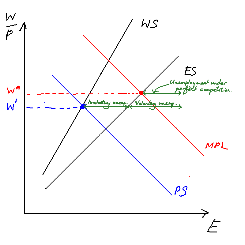
The ES, WS, PS and MPL pin down the level of real wages at a certain level of output.

In a competitive labour market, the demand for labourers is given by the MPL. The supply is given by individuals' utility functions, but we shan't go into that here.

The intersection of employment supply (ES) and employment demand (MPL) is the equilibrium level of employment in a competitive market. Note that employment demand is downward sloping due to diminshing returns (see assumption 1).

However, in this model, participants have market power (assumption 3). Labour unions can sign labour contracts that give them wages above the competitive wage. This is called the wage-setting curve (WS) that lies above the ES curve.

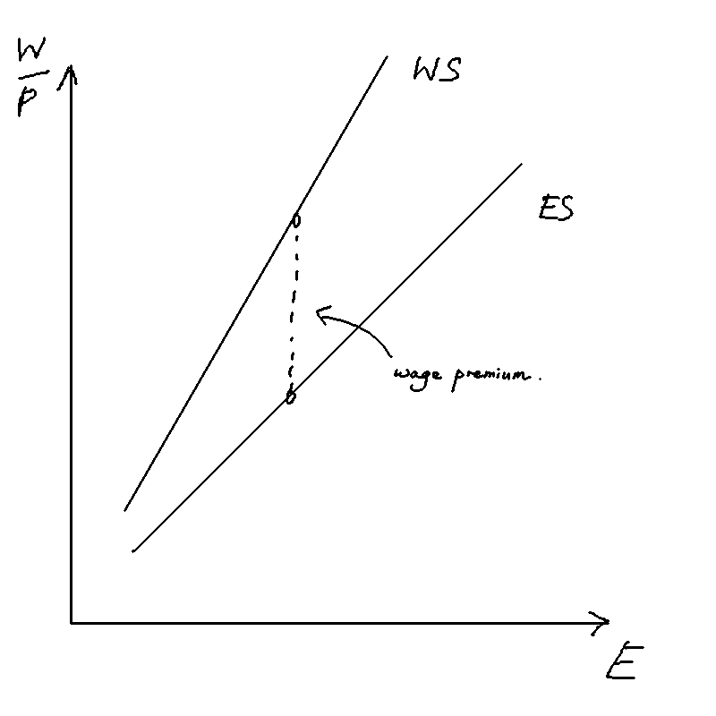
Similarly, there is a price-setting curve (PS) that lies below the MPL curve. The intersection of these two curves is the equilibrium level of employment

Involuntary and voluntary employment

Voluntary unemployment: people who are not willing to work at the prevailing market wage Involuntary unemployment: people who are willing to work at the prevailing market wage, but cannot due to the fact that the labour unions have priced them above that.

• No involuntary unemployment if workers have no market power

Effect on wages ambiguous

The effect on wages is ambiguous. It depends on the relative slopes of the WS and PS curves.

Compare these two images.

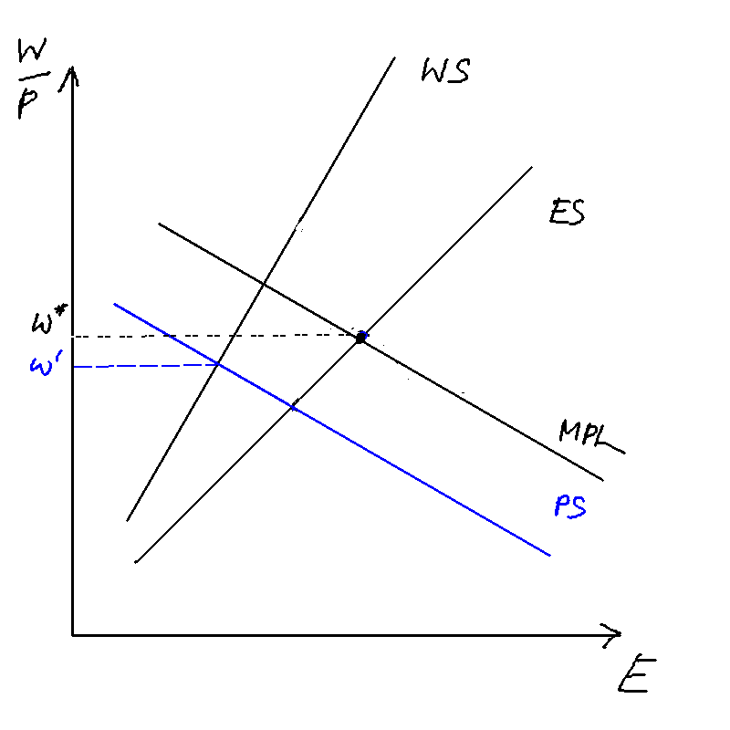
In the figure on the left, the competitive equilibrium's wage w* lies above the wage that was gotten in the noncompetitive equilibrium. In the figure on the right, the reverse is true.

The PC curve

$PC: \pi_t = \pi_t^E + \alpha(y_t - y_e)$

In the case of adaptive expectations,

$PC: \pi*t = \pi*{t-1} + \alpha(y_t - y_e)$

Microfoundations

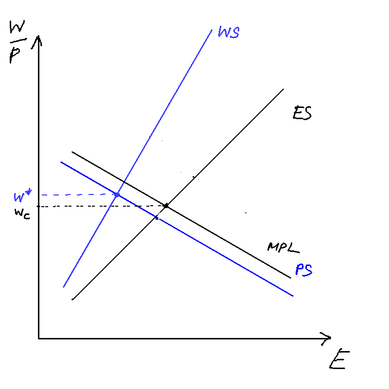
The Phillips curve is gotten by the interaction of the WS and PS curves. The Phillips curve states that inflation in this period equals expected inflation this period, plus a shock from the output gap. But why would the output gap affect inflation? We use the WS and PS curves to explain.

With the WS and PS curves in place, we can begin to understand the Phillips curve.

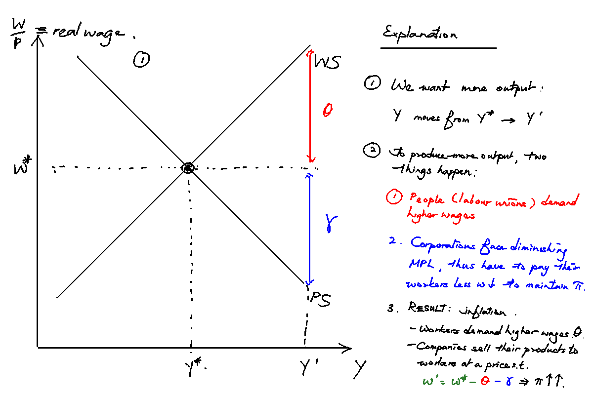
The figure illustrates. Suppose we want to raise output from Y* to Y'. Well, two things will happen:

1. Labourers will demand higher wages to work more
2. Due to diminishing returns, MPL will fall: companies are willing to pay less.

Labourers will demand more to work. They'll want a real wage increase of $$\theta$$ (in red).

The companies pay that wage. But they have the last laugh---they simply set the price of their goods higher, so that they make the same profit! Specifically prices will go up such that labourers' real wages are eroded like so.

$w^{'} = w^* = \theta - \gamma$

(remember from assumption 2 the economy is made up completely of companies and labourers, and labourers buy the goods the companies produce)

Therefore, prices go up == inflation.

The coefficient $$\alpha$$ in the PC depends on the relative steepness of the WS and PS curves. The steeper both of them are, the larger the gap between the two curves, the larger the coefficient, and the steeper the PC will be.

The MR curve

Central bank's loss function:

$L = (y - y_T)^2 + (\pi - \pi_T)^2$

The MR is the central bank's best response to the Phillips curve. That is to say, it solves the optimisation problem

$L = (y - y_T)^2 + (\pi - \pi_T)^2 s.t. \pi*t = \pi*{t-1} + (y_t - y_e)$

So we substitute the PC into the loss function, differentiate, and rearrange to obtain

$\pi = \pi^T - \frac{y_t-y_e}{\alpha \beta}$

a, alpha and beta

a : Found in the IS curve. Measures how responsive the economy is to interest rate changes. - For instance, economies credit-constrained consumers will have higher a.

$\alpha$: Found in the Phillips curve. It measures the relative steepness of the WS and PS curves. - Stronger labour unions or firms with more market power increase $\alpha$.

$\beta$: Found in the central bank's loss function. Measures how inflation-averse a bank is (how much output it's willing to give up in order to decrease inflation). - A more inflation-averse central bank will increase $\beta$.

The effect of these coefficients on MR

• $\beta$: Makes MR less steep. A highly inflation-averse CB (high $\beta$) is going to be willing to cut a lot of output to decrease a little bit of inflation. At the limit, where $\beta \to \infty$, the MR is a straight line: the CB will literally do anything to prevent any deviation of inflation from target.
• $\alpha$: Makes MR less steep. A greater $\alpha$ means that a small change in output gives a huge change in inflation (remember that $\alpha \propto \theta + \gamma$. So the CB gets more "bang for your buck": it's thus very willing to adjust output in order to reduce inflation, because it can do it relatively cheaply.

But note that the effect of $\alpha$ on policy path is ambiguous

Supply shocks

TODO

Supply shocks are cost-push shocks. They affect the PC curve.

Let's examine the case of a temporary positive supply shock.

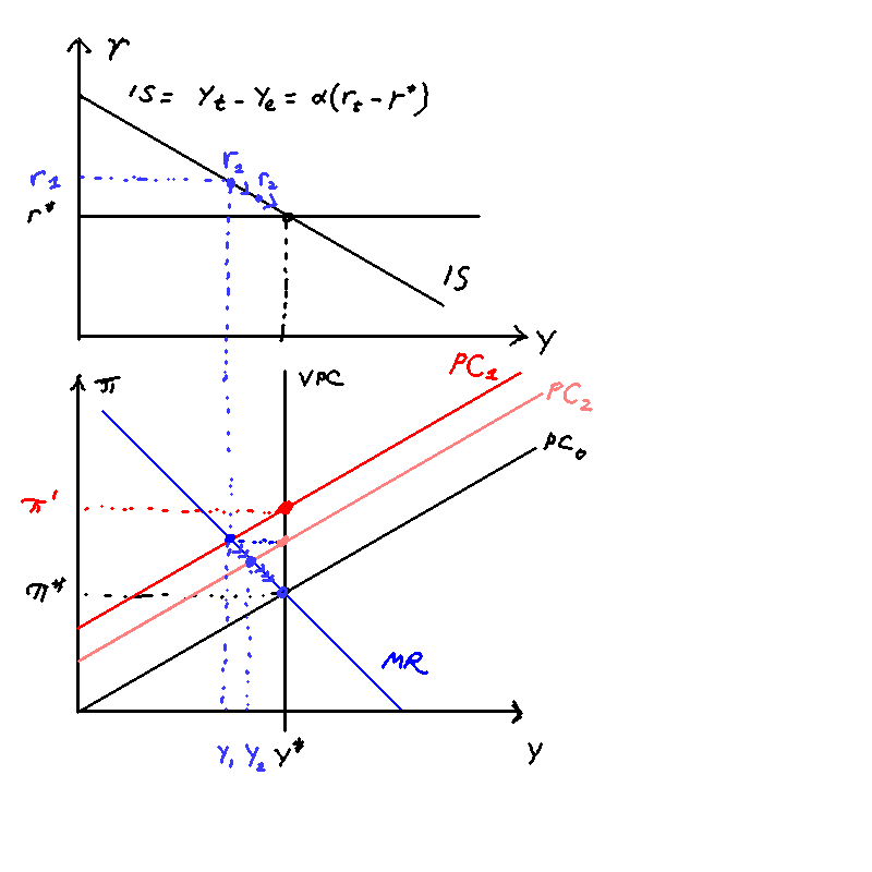
• $t_0$. The economy is at steady-state with $Y = Y^{*}, \pi = \pi^{*}, \text{and } r = r^{*}$. A supply shock causes prices of goods to increase unexpectedly. The PC moves up from $PC_0 \to PC_1$. Immediately, the central bank raises rates from $r^{*} \to r_1$ in order to cut output to Y_1. But as monetary policy operates with a lag, this change doesn't take effect until the next period.
• $t_1$. The PC remains elevated at $PC_1$. But the interest rate now takes effect and causes output to fall from $Y^{*} \to Y_1$.
• $t_2 \text{ onwards}$. The PC falls from PC_1 to PC_2. The central bank lowers rates slightly. There is a protracted adjustment of interest rates and output back to their equilibrium values.

Demand shocks

TODO

Demand shocks affect the IS curve.

Let's examine the case of a temporary positive demand shock.

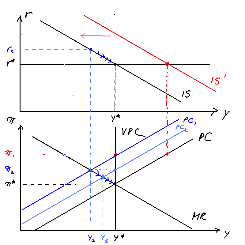
• $t_0$. The economy is in eqm. A positive temporary demand shock hits, causing the IS to shift from $IS \rightarrow IS^{'}$. Inflation rises to $\pi_1$. The central bank immediately hikes rates to $r^{'}$, but as monetary policy operates with a lag, this change doesn't take effect until the next period.
• $t_1$. The IS curve goes back to normal, but due to higher inflation expectations the PC shifts upwards to $PC_1$. Due to the central bank's hiked rates, however, inflation decreases from $\pi_1 \rightarrow \pi_2$.
• $t_2 \text{ onwards}$. There is a protracted adjustment of interest rates and output back to their equilibrium values.

How the central bank can do better if it expects the shock

TODO

If the central bank expects the shock, it can cut/hike rates one period before the shock. The moment the shock hits, output is already stabilised --- as though the shock never existed.